From S3 to GPU in One Copy

Before I get into anything, I want to show you this video. Not specifically like what's playing in the video, but how we produce this video. Because this is not backed by a regular MP4 file in some main disk, but this is actually a visualization of a file scan. What I mean by this is we have a Vortex file, Vortex being a columnar file format. It has three columns, one per color. Each column would then have a row per frame of this video. Each frame would include around 8 million pixels, because it's a 4K video. Then we then process this data, which is three columns, around 8 million pixels per frame, 60 frames per second, so around 13 gigabits per second, from S3, through the network card, over the CPU, and to the GPU. The GPU is seeing this data this fast, but we want to see what's happening in the GPU, we want to visualize that.

We can't downlink that much data to our laptops, so because it's already in the GPU, I'm using the GPU itself to re-encode it into H.264, wrap it into TCP buffers, send it over my SSH tunnel, and we can display and see what's happening. Now have a look at this. This is the same video, but this doesn't have any post-processing on it. This is actually a visualization of a column pruning, or projection pruning, where we only select, in our projection expression, one column, and only the bytes that are associated with that column are flowing through the same pipeline, keeping the same bandwidth, and then ending up with the video that you were seeing before.

Today I want to talk about how this is possible, and the technologies that enable us to do this. I'm Onur. I work at SpiralDB. I help maintain Vortex, which is an open-source file format that is under the Linux Foundation. I want to talk about what makes Vortex special. I'll start with why we need this speed in the first place. I'll then move on to Vortex itself, explain some of the main topics around Vortex, layouts and arrays and the scan itself, and then end with what is possible.

To start with the problem, why we need the speed. Because you have some GPUs that you hired and you want to use them. GPUs are expensive, and then each time they're idling, it's expensive, and it's an opportunity cost of not doing valuable work. I want to tell this like we have two types of taxes that we pay when utilizing GPUs. The first one is a movement tax. Getting the data from some source that you have into the GPU is not trivial, and it's not really cheap. If you use web dataset for training, or for example, MosaicML's streaming dataset, then they go more or less these steps. For example, let's say your data is in S3. You fetch from S3 into the disk, into NVMe. From NVMe, you read compressed bytes into your RAM. You decompress on the CPU, and then send those decompressed bytes over the host of device link, PCIe, to the GPU.

This not only has many steps that you have to follow through. If you zoom in into the supported bandwidth per connection, you can see that we are bottlenecked mainly by CPU decompression, and the NVMe throughput. The reason why they all persist into NVMe is the main consumer of this pipeline is PyTorch. PyTorch is Python. Python doesn't like multi-threading, so therefore we use multi-processing. Each worker doesn't want to step into each other's toes, so they want to deduplicate the downloads, so they persist the shards on the disk. Ideally, we want this pipeline to look more like that, where you fetch from S3, eliminating the bandwidth bottlenecks through the network card speeds and the PCIe speeds to the GPU. Then, further, you want to use the right compression that enables you to decompress in the GPU, the parallel compressions, and GPU can decompress much faster than CPUs. You're not only eliminating the bottlenecks you had in NVMe, and you're streaming much faster now, you're streaming maybe 50 gigabits per second, but those bytes are compressed. If you pick the right compression, effectively, this pipeline runs through 10 times faster than the actual compressed speed. That was movement.

There's another tax I want to talk about, which is decision. It is when you want to iterate on your training workload. You've loaded from your source into the GPU, and maybe you did some preprocessing to your training, then you want to evaluate the results. What you want to then try, for example, is a new data mix, or you want to change the curriculum. You want some new filter on this data. With the current tools we have, you have to reprocess the entire data, probably re-tokenize, reshuffle to get the right order, and then load again to your source, which might be S3, might be somewhere else, but this is slow. If you look at the hypothetical pie chart of your percentage of time spent, you want to maximize the gray, where you're thinking, and the green, where your GPU's working. Everything else is overhead. You want to turn this into that, where you load from your source into the GPU without wasting much time. Then once you evaluate and decide you want to change something in your input source, then you just change your scan. You just give a different query, a different filter. You don't need to reprocess. Then you immediately can start training for your next iteration.

How does Vortex, using a different file format, enable all this? Vortex, to give a quick overview of what it is, it's a columnar file format. It is similar to Parquet, but it's also much different than Parquet. It has an extensible spec, a minimal spec that you can plug in into various points. It has a separation of logical types versus physical types. That's one of the main differences from Parquet, is that Vortex doesn't have a notion of tying the types themselves, like integers, into how they're encoded on disk. It's up to you, it's decoupled. It does as little as possible, as late as possible, saving a lot of memcopies for materializing intermediate results, and leveraging from query optimizations. Then it can push through most of the projections, filters, and aggregation from your compute engine into the file format itself. Also, the way it does compression is different.

It doesn't use block compression that loses the meaning of the underlying data. It does use lightweight and cascading encodings that can also give a similar compression ratio, but more importantly, they allow you to do compute on the compressed data. You can do random access, you can do aggregations. Some of these computes can be even faster than doing it on the decompressed data itself. To give some concrete numbers versus Parquet, this S3 to GPU scans that we are showing is around 30 times faster. Thanks to the encodings and the compression Vortex has, it's around 100 times or more faster than Parquet in random access.

What does the file look like? We will approach this from a file reader's perspective. There's a Postscript that's fixed size, you read it, it has a lot of pointers into other sections of the file. There's a footer. The footer itself is a legend, it's a bill of materials of what you expect to see in this file. You have a list of arrays and you have a list of layouts. Arrays are how you encode the data itself in Vortex, and layouts are like the logical plan. They are the I/O layer of pruning. We will dive into that later. These are showing you the main plug-in points. If you have a new array of a new layout, you just add it here, and you have the logic in your reader, then Vortex will delegate to your reader to do what you want to do. Thirdly, and maybe most importantly, it's the list of segments that you expect to see in this file, and the segments are the majority of the file.

They have the array data themselves. They come with triplets, so offsets, length, and alignment. They're pointers, but they also have alignment. Alignment is important to bake in the file, we think, because if you have the alignment, you know that if you want to use SIMD operations or GPU kernels when you load this, if you know the alignment beforehand, in your receiving buffer, you allocate that buffer with the right alignment, so you don't need to copy, just to dispatch the compute on top. I've talked about arrays and layouts, but what are layouts? Layouts enable you to prune those segments as quickly as possible, given a filter and projection. They are like the logical plan. They are also very minimal. This is the entire flat buffer definition. The only two maybe important points I want to touch is the last two fields. It has the children, which is an array of itself, so it's a tree, and each node in this tree has segments.

Segments is a list of integers, and those integers point to the offsets of segments. We know from the footer where they are in terms of pointer, like exact byte ranges. Each node in the layout tells, I am responsible for reading these segments, and give me a filter, and I'll tell you which of these segments I'm responsible for, you have to read.

To give an example on how layouts work, let's start with a schema, for example. We have the root layout. It has two columns, a name, string, an age, integer. The StructLayout only tells it, I have a child per column, so you expect it to have two different children, one per column. Each of these is a ZonedLayout itself. ZonedLayout is interesting because it not only contains the data as segments, it also contains another segment that is a summary statistics of the data that you expect to read. That's also a segment itself. When you read that segment, it's a zone-map. A zone-map is a Vortex array by itself, but it does have a per row range in the actual data, and has columns of statistics, like min, max. The data is then just a concatenation of multiple segments. It's a way of breaking it down into smaller arrays when you want to read them.

How does this work, then? Say you have this query. You want to get the name column, but you only want to get the rows where the age column is greater than 30. You start from the root. Root knows it has a projection and a filter in each column, so it delegates into each ZonedLayout through this. The age will receive a filter, and it will then initially load the zone-map, check the zone-map, check the filter, find which segments in this data passes the filter. Let's say the last segment passes the filter, so then it returns the last segment. We also get the name column to return the last segment, because that's the actual data we need. Do the actual filter on the actual rows, and return the rows that we need. By reading the zone-map and only 30% of the segments, you can satisfy this query.

Maybe this is a more detailed view. The center is the zone-map. That was a segment. We read it. We deserialized it. It's an array. It has one row per row range, and we have the filter. By just looking at the max value, we can prove that only the last row here can have any rows that match this filter. All the others you don't need. You read the entire chunk. That's the Vortex atomic unit of reading. It's a segment inside. Then, what's neat about Vortex is the compression we have is sliceable. You don't need to decompress everything. You slice it first, and then you only decompress the rows that match the row range we have it. The last 8k rows is decompressed. That is like doing as little as possible and as late as possible. The difference between chunk granularity and row granularity is also, I think, important to mention, because these serve different purposes.

Chunk granularity is an I/O concern. It deals with what type of I/O source you have, what is bandwidth and latency characteristics, so you can tune them in Vortex. The zone granularity itself is a compute concern because, depending on your architecture, you might have different wider SIMD registers that you want to use, and those play well with different lengths of data that you have. You can tune them as to your liking with Vortex.

We talked about reading the segments and layout is helping us prune to the segments that we want, but what do each segment contain? They contain a serialized, most likely compressed Vortex array. A Vortex array, I want to also explain with an example. Let's say we have this array. It's an array of arrays, so the element is a list itself. The elements inside the inner lists are strings. We want to encode them and compress them as much as possible while keeping the meaning. We can start with a ListArray that's similar to Arrow. It basically flattens the values and saves the flattened values as a values child, and then it keeps the inner brace locations because it removes them while flattening, it loses the information, so it keeps that information into the offsets child. Any two consecutive offsets would point to the inner braces of an inner list location.

You can see this is also a tree. Now we have the ListArray, but two children are also arrays themselves. We can go on further, we can compress further. For example, the values child has only three unique elements so we dictionary encode them. Dictionary encoding gets the unique values and stores them as children, so like in a values child has one city appearing once only, but you then encode the repetition of the original array as the indices that point to the values child. Then you decoupled the values themselves and the repetition into separate children. Then you can continue further because the codes now have contiguous repeated values, which are called runs. You can run length encode them, or in Vortex, more specifically, run end encode them, meaning you get the values that repeat, save them as a child, 0, 1, and 2 are the values of each run here, and then you also encode which offsets in the original array these runs end, so the actual indices that end.

With this, we have the string values as a child, but we also have multiple integer values that we have, and we can see that all of these values are really small. The values child of run end, they're all smaller than four. Four is second power of two, so you can encode each of them in two bits. The ends and the offsets are all less than eight, so you can use three bits to encode them. You bitpack all of this integer data you have and end up with the actual bits on disk like that. That means this is total 30 bits or so, so this is less than one integer. It's less than 4 bytes. Then using this information, you are storing all the repetition and nested structure of your input array, and you only store the unique elements once. We can further compress this. We have FSST, for example, is an algorithm that extracts the common substrings and then further divides into arrays.

For this example, I think this gets the point. I want to separate these two things into two ways. You have the arrays, which is a structure, which is how you encode this segment. Then, it is important because this is what you would use to dispatch compute. On the right-hand side, you have the data. I want to think of these two as the control plane and the data plane, and that will be important in the scan, which we'll go into later, but before, I want to mention one more thing. Having this array tree on hand and having this data as pointers somewhere in some location, you can dispatch compute without decompressing. For example, I want to get a random read. I want to get the second element of the first list. If you get that query into the ListArray, ListArray knows that it can binary search the offset child to find the actual location, then does propagate that to the flattened values child because it now knows the actual location.

DictArray can do the same for code, and then substitute with the right value before returning. Also, I mentioned some compute you can run on the compressed data might end up being faster than running the compute on decompressed arrays, like summing, for example. Summing requires, on a decompressed array, iterating through each element and summing the values. If you have a run end array, that's just multiplying with the lengths of each run, and then per run, you are summing the total result of the multiplication. It's a lot faster to run the compute on compressed data.

Back to the separation. The control plane shows you the amount of information you need in a compute engine so you can dispatch work on the data itself. The data plane is the information you have to transfer to your compute engine. These serve different purposes, and we don't want them to step in each other's toes. How do we do this? Vortex has a scan that tries to maximize this throughout. The way it works is it tries to maximize the I/O engine's work and the compute engine's work to be busy all the time. Then, scan is the orchestrating layer. The orchestrating itself also wastes compute and has to dispatch work, reconstruct the array trees, and then follow the array tree logic all the way to the end. The I/O layer then gets some bytes to the compute source, returns the pointers, the scan then dispatch work on those pointers.

A small detail, but compute also can request more segments because, for example, in the query that we initially did, select name where age is greater than 30, you don't know if you need name column before executing the age filter. It could just be pruned all together so you don't end up getting those segments. Say we have a query in the scan, and then we have the layout in the scan so we know which segments we need to fetch. Those are transferred into byte ranges, and these are byte ranges that you want to get from your source. Each individual byte range might have a latency, and depending on what source you're reading, you don't want to dispatch each individual byte ranges by itself. We have a coalescing layer on top, and coalescing means if two byte ranges are close enough sufficiently, you merge them and then have a single byte range.

You get extra bytes in between, but because you pay the latency once and get the entire throughput, it works on your benefit. This is source-dependent. NVMe is happy with some coalescing configuration, but S3, for example, might require a lot more. S3, you can do 16-megabyte segments because it's a huge throughput with huge latency. Once you get the segment request and then have the byte ranges, you then dispatch work on them. It's a CPU scan. This work is done when you have the bytes on RAM. Then the work you dispatch is regular Rust functions like slice, projection, filter, any compute that the input query wants you to do. That was CPU. Most of the things stay the same when you are scanning to the GPU. The scan orchestration stays the same, the coalescing layer stays the same because we still need those byte ranges, but now the I/O plane has to ship these buffers all the way to the GPU and return pointers to the GPU. That's when its job is done. The compute, now instead of dispatching Rust functions, it does dispatch CUDA kernels, but everything else is the same.

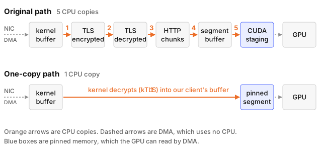
We have a buffer pool in the middle, and I want to explain why we have a buffer pool in the middle. This is the lifetime of a byte range through a scan from S3 to the GPU. Initially, when you request bytes from S3, it lands on the kernel, receive buffer. This is a direct memory copy, so it's not an actual copy, it's the first place that these bytes land from the network card, is this kernel, receive buffer. It immediately copies the ciphertext, still in a TLS encrypted form, into the userland, one-to-one. Then we are in our HTTP libraries land where we use Rust TLS and request. Rust TLS decrypts it into plaintext copies, that's one copy, and then it's still TCP, we want to get the HTTP body out of it, so the request layer deframes it, gets the body into its own buffer, then finally it arrives to our own Vortex land.

Because these yellow buffers are all streaming, because they're multi-part GET request, we have to aggregate them because we want the segment, we want a contiguous byte range. We aggregate them, so we have to copy one more time, but that's the only copy we do. We receive these chunks as a streaming fashion, and then we accumulate them until the request is done. Immediately after this is done, we dispatch the CUDA. We do CUDA async copy and expect it to land on GPU, but unbeknownst to us, internally, CUDA does another copy. It does another copy because it requires some alignment rules from us. Basically, the buffers you can copy to the GPU from the host has to be pinned and page locked, meaning it should be outside the operating system's virtual page system, so then the copy, if the buffer gets paged out during the copy, GPU doesn't segfault and stays happy.

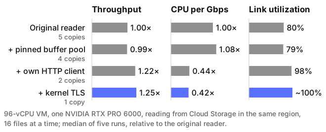
Before diving into how we can reduce the copies, I want to mention one more thing. The memcpy cost is what's important to us. The unit is a core per gigabit of bandwidth you can sustain. It's important because this core budget is also used by the orchestrating layer in scan, and also compute if you're doing the compute on the CPU. It has the opportunity cost, because you have limited CPU, if you're just wasting it on memcopies all around, then you slow down your own bandwidth. It's like a double-edged damage, so you want to reduce this as much as possible.

How can we reduce this? Initially, we start with the CUDA bounce buffer because we know the requirements. We can satisfy those requirements on our own buffer that we accumulate the HTTP buffers into. We have a pinned buffer that we use, and then we then call CUDA async copy on it. It doesn't use a bounce buffer, and this goes directly into the GPU. Further, because allocating these are expensive, we keep a buffer pool around to amortize the allocation cost. The way we reuse these buffers is when you dispatch the CUDA copy, you append the CUDA event after that CUDA stream. You append an event. Once that event fires, you know everything that comes before it is complete, so then you can safely reclaim the buffer because that means the transfer is complete, and you can reuse that same buffer for next copies in your pipeline. This reduces the cost a bit, but we need to then look to the left, to the HTTP land, to get rid of some of the copies.

One thing you can do here, if you have a sufficiently high Linux version, you can use a kTLS, kernel-side TLS decryption. That pushes the decryption into the kernel, and because the kernel was immediately copying into the userland, then it doesn't need to do it anymore because now it's decrypted, and then the decrypted can be in place. The decryption can be in place in the receive buffer itself, so it saves one copy. There's one caveat that the Linux ciphers are mostly not really that up-to-date in kTLS, so they might not end up using the widest SIMD registers your machine has, but still, the memcpy saves here because we reduce one copy, offsets that deficiency, in a way, so we still keep this kTLS in this land.

What else can we improve? We can improve more things on the HTTP side, but for this, we need to do bigger changes because there is no low-hanging things we can do here. If you do bigger changes, namely writing your own HTTP client, then it pays off well, because if you write your HTTP client, you control which buffers you give to kernel. If you do it, you can use the already pinned and page locked Vortex buffer you have to accumulate and deframe on the fly in the same buffer. Once you get the decrypted bytes as a stream in the multi-part GET request, you keep allocating them into the same buffer you already had to be ready to be sent to CUDA. Then when the multi-part GET request is complete, you dispatch to work, and you cycle these buffers, so with one copy, you go from S3 to GPU, and you have very little CPU overhead during the entire scan.

There's one more iteration of this, but you have to get rid of TCP. If you have a very expensive and tedious setup, but really performant and cool RDMA object store in your hands, then you can use RDMA protocol, which is different from TCP, that it doesn't have to go to the kernel sockets layer. It can bypass the CPU entirely because it works as two peers connected via some sort of fiber, can be PCIe, can have some network connection, can be in between, but they can read and write from each other's memory regions. If you have this ability, then the GPU itself can dispatch the I/O request on your behalf. If it does it, it not only bypasses all CPU, it even bypasses the PCIe hub of your CPU, because these boxes come with multiple GPUs and come with many network cards. Most often, each GPU has an associated network card, so the RDMA would flow through from the GPU into the nearest network card, bypassing your CPU PCIe hub all together, so it's basically free. The CPU doesn't even know what's happening. For this, the network card also needs to be smart enough, but most boxes that come with high-end GPUs have that network card in place already.

With all that, let's revert back to the video. Now, you can see there is some byte range coalescing, so we have a filter or projection. In this case, we have no filter, and we SELECT *, essentially, all columns, red, green, and blue. They all go through this coalescing layer. Then we fetch these bytes from S3, and then we cycle the byte buffer that we read them through, and they go only one copy into the GPU, and then the GPU processes them as 15 gigabits per second, 4K, 60 hertz, and then we stream it back to see what's happening. What's also cool about this, because while we have it, we can change the filters and projections. We can do, for example, this. This is not a post projection. This is actually a combination of a projection and a custom Vortex expression. I have written this custom expression called quantise, and I've written a GPU kernel for it, which is very basic.

Quantise just gets the colors, each pixel value is 0 to 55, and then it snaps it to three levels, basically, depending on which level it's closest to. You get this effect of having only three columns. We also pruned the blue column out of the way, just for fun, so it's more yellowy, but also this discretized footage we have. This is, importantly, mostly handled by Vortex orchestration. You don't tie this kernel at the end yourself. You just say that I want this query, and the scan orchestration takes care of appending your kernel, and then dispatching work onto your kernel, and then you can keep the same throughput. Or you can do something like this. This is a bit jarring to watch, because the video skips all over. The way this works, remember I told you when we have this file with three columns? This file has four columns, and the fourth column is whether the frame has a cyclist or not.

I've run this object recognition algorithm per frame, and then we now have this has_bike Boolean column, as the fourth column, and I'm filtering to only the frames that has a bike in it. The way this works is because each frame is huge. Each frame we have is 8 megabytes. We can afford to have a zone per frame. In the layout level, we have a zone-map that is as granular as it gets. We have one row per frame, and so we can prune each individual frame that doesn't have a bicyclist on it.

Maybe what's more important to talk about here is all of these changes don't affect throughput. You can come up with an arbitrary filter. You can come up with your own projection. You can combine them, but you can keep the same throughput, and you only read the data that you need. Remember I told you the videos were 60 frames per second because I was intentionally slowing them down. Normally, when you let them loose and then write it to like a file, then we can stream 240 frames per second, because I was pacing the video so we can see it at 60 frames per second, but we can sustain 60 gigabits per second end-to-end with Vortex.

I want to talk very briefly on what you can do with Vortex if you want to customize it. Remember I told you, you can have your own arrays and you can have your own layouts. A layout is responsible for I/O and then logical plan and then pruning and all that stuff, but it's also responsible for placement. There's nothing in Vortex file spec that enforces you to be in the same physical file. You can separate your segments into two. You can get the pruning segments and store them in Redis, and you can get all the array segments in S3. Redis has one-hundredth of the latency of S3, so you get pruning nearly immediately compared to the numbers you would get with S3, and then you get the S3 throughput on streaming the data to the end. Or, say you have this giant instance with multiple high-end GPUs but a single CPU, and then you have this GPU analytics engine that you shard the data into individual GPUs, and then you run a scan, and then dispatch the scan into individual shards.

What if the query has an aggregation? Then you need to aggregate all of the results into a single GPU. You can model that aggregation as an RDMA scan, because GPUs are connected to each other with an extremely fast fiber called NVLink. It can sustain tremendous speeds. You can scan from one GPU to your central GPU to aggregate, and you can scan in terabits per second for the segregation.

That was Vortex. I wanted to talk about how it allows you to change your filter, to change your data mix and not reprocess everything over and again. I also want to mention that you can read from S3 into GPU around network card speeds. It can be 60 gigabits per second, can be more if you have a stronger network card. You can read from RDMA sources to your GPU at whatever PCIe connection you have, and that can be 500 gigabits or terabits with the newest PCIe.